PID Control (with code), Verification, and Scheduling

Hi all
PID controllers are the workhorse of the controls world. PID controllers have the goal of taking some error in your system and reducing it to 0. While there are many other control strategies out there PID is probably the most common (unless you count human control) outside of just setting a setpoint. There are many advanced control strategies out there but in most cases they will do similar or worse than a PID and be much more complex. When the other methods do better it will often only be by a small amount. One exception is if you have a model of the device and its operating conditions you can create a feed forward controller (good for PhD students) that performs better. However in many cases using reactive control with a PID is the easiest and fastest approach to implement.

When we talk about PID control you should remember that each of the letters represents a different mode of the controller. The P is for proportional element, the I is for the integral element, and the D is for the derivative element. Each element has a “term”, that gets multiplied with those elements. We use K to be a generic constant value, so the constant terms (or gains) are K_P, K_I, and K_D respectively. Depending on your application you may or may not have all three of the terms. In many application you will have just PD or PI terms.

So the basic question is: How do you convert the error in a system to form a better new command?

Click image to see clearer/larger version of equations.

There are many forms of the PID controller. But here are the two that most people will care about:

Note: e and e(t) are the error terms, this is defined as: e = desired_value – actual_value. Often the actual_value is coming from some sensor that you have to detect the current value.

The first is in continuous time:

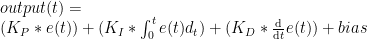
The second is in discrete time, which is what is more commonly used in computer controlled applications:

And here is some pseudo code for the discrete version of the PID controller:

error_prior = 0
integral_prior = 0
K_P = Some value you need to come up (see tuning section below)
K_I = Some value you need to come up (see tuning section below)
K_D = Some value you need to come up (see tuning section below)
bias = 0 (see below)

while(1) {
error = desired_value – actual_value
integral = integral_prior + error * iteration_time
derivative = (error – error_prior) / iteration_time
output = K_P*error + K_I*integral + K_D*derivative + bias
error_prior = error
integral_prior = integral
sleep(iteration_time)
}

While the discrete approach is more useful from an implementation perspective. When it comes to understanding and tuning your controller the continuous approach is important for you to understand.

Also while you usually do not see the bias term added to the filter, I like to put it in just in case everything else sums to 0 and you still need motion, I will not have a 0 as the output. This is not strictly needed but it is nice to have in many cases. For example if a wheel needs to continuously be rotating and the PID is just to maintain a given velocity.

The Terms

So now we know the form of this controller we can look at what each term does.

Proportional Term (K_P)

The proportional term is your primary term for controlling the error. this directly scales your error, so with a small K_P the controller will make small attempts to minimize the error, and with a large K_P the controller will make a larger attempt. If the K_P is too small you might never minimize the error (unless you are using D and I terms) and not be able to respond to changes affecting your system, and if K_P is too large you can have an unstable (ie. weird oscillations) filter that severely overshoot the desired value.

Integral Term (K_I)

The integral term lets the controller handle errors that are accumulating over time. This is good when you need to handle errors steady state errors. The problem is that if you have a large K_I you are trying to correct error over time so it can interfere with your response for dealing with current changes. This term is often the cause of instability in your PID controller.

Derivative Term (K_D)

The derivative term is looking at how your system is behaving between time intervals. This helps dampen your system to improve stability. Many motor controllers will only let you configure a PI controller. In some cases this can be negative.

Which permutations of P, I, & D do I need?

In many applications you will not use all 3 terms. So why not just always use all 3 terms? The fewer terms you use the easier the controller is to understand and to implement. Also as you will soon see some modes can cause instability (ex. extreme vibrations) in the controls.

Just about every filter will have the P term. So lets just assume that K_P is in our filter. Now the question is do I want to add just I, just D, or both into my filter.

If you want you can only have a P term. This is the simplest type of controller to tune since you only are playing with one value. The downside is that your controller will not smoothly correct itself for sudden and sustained error.

If you add a D term you will be more susceptible to noise and random values. So if you have very noisy data, or random impulses that your sensors measure, you might want to leave the D term out. The downside of leaving the D term out is that you are not responding to those random values that might be legitimate, so you will have a slower response time. An example of this is if your motor hits a rock it will take longer to increase your commanded value since you are not looking at how the error is changing with time. However if you are working on a robotic arm you might want the D term so you can quickly respond to changing forces.

The I term gets tricky. In many cases you will want the I term so you can recover from error that is slowly accumulating. The downside is that the I term is slow to respond. This slowness can lead to instability in your control.

How to tune your filter?

Tuning a filter can be difficult since a device (say a motor) might need to respond to different conditions. For example if you tune your motor with no load it might not perform optimally with a load; and if you change the load you might need a different set of values to get optimal control. So often you are trying to find a set of parameters that works best in all cases and not necessarily optimal for any given case. There is another approach where you get different constants (the K values) to use in the filter and you choose which set to use based on the actual values in the system.

There are many ways to tune a PID controller. The two best ways that I know are manual (I know people don’t like manual things that relies on having an expert around) and Ziegler–Nichols method. With that said I have found that I can get better results by manually tuning a system, however you can use the Ziegler–Nichols method as a starting point. (The next two sub-sections are mostly taken from wikipedia).

Manual Tuning

If the system is online, one tuning method is to first set K_I and K_D values to zero. Increase the K_P until the output of the loop oscillates (or just performs well), then the K_P should be set to approximately half of that value for a “quarter amplitude decay” type response. Then increase K_I until any offset is corrected in sufficient time for the process. However, too much K_I will cause instability. Finally, increase K_D, if required, until the overshooting is minimized. However, too much K_D will cause slow responses and sluggishness. A fast PID loop tuning usually overshoots slightly to reach the setpoint more quickly; however, some systems cannot accept overshoot, in which case an over-damped closed-loop system is required, which will require a K_P setting significantly less than half that of the K_P setting that was causing oscillation.

Ziegler–Nichols

Another heuristic tuning method is formally known as the Ziegler–Nichols method, introduced by John G. Ziegler and Nathaniel B. Nichols in the 1940s. As in the method above, the K_I and K_D gains are first set to zero. The proportional gain is increased until it reaches the ultimate gain, K_U, at which the output of the loop starts to oscillate. K_U and the oscillation period P_U are used to set the gains as shown:

Verifying Control Parameters

You can verify that the selected gains are good by looking at the output waveform when a step command is applied. If there is a lot of initial ringing (constant changing) or overshoot in the beginning of motion, your gains are probably to high. If the initial command is slowly reaching the desired output you might need to increase your gains.

Plots showing common tuning problems followed by a good response curve. The blue lines are the command, and the red lines are the actual motor output.

In the image above starting from the left we can see:
1. Overshooting of the output motion, with a little signal ringing as it settles to the command. A little overshoot is often fine, but we do try to minimize overshoot while still having a responsive system.
2. Slow response of the output. We might want a faster response so the system will be less sluggish. As you make the system less sluggish you often increase the overshooting and potential for instability.
3. Highly unstable. Starts with a bunch of oscillation, followed by a large spike in command output. We want to avoid this!
4. Finally this right-most plot looks good. The motor output is directly on top of the commanded motion, with a very slight overshoot (if you look close).

The next step in checking the stability of the system you just tuned can be Bode plotting. Click here to learn about it

Gain Scheduling

In the simplest terms gain scheduling lets you pick different sets of terms based on the performance of the system. So you could say that if the speed is less than or equal to some value use one set of PID terms, if the speed is greater than that value use a different set of PID terms. This is often used in non-linear systems so that you can simplify it to several (almost) linear portions. This is also good if there is some region of the controller where you need to be more aggressive.

Practical Programming Tips

PID’s (and other controllers) can cause very abrupt changes to your commands. One way to mitigate this is by using trapezoidal control (not to be confused with trapezoidal commutation). By setting acceleration and deceleration rates we can make sure the control is smother and less abrupt.

Another useful tip is to remember to set a min and max command that can be sent to your motors. This will prevent the PID controller from generating bad/extreme commands to your motors.

Many motor controllers let you specify the above acceleration, deceleration and limits. Saving you from having to implement this from scratch.

I hope this was useful, and happy tuning!

Liked it? Take a second to support David Kohanbash on Patreon!