

Hi all
Here is a quick tutorial for implementing a Kalman Filter. I originally wrote this for a Society Of Robot article several years ago. I have revised this a bit to be clearer and fixed some errors in the initial post.
Enjoy!
Note: The post has been translated into Russian here and is hosted by Everycloud
Introduction
Kalman filtering is used for many applications including filtering noisy signals, generating non-observable states, and predicting future states. Filtering noisy signals is essential since many sensors have an output that is to noisy too be used directly, and Kalman filtering lets you account for the uncertainty in the signal/state. One important use of generating non-observable states is for estimating velocity. It is common to have position sensors (encoders) on different joints; however, simply differentiating the position to get velocity produces noisy results. To fix this Kalman filtering can be used to estimate the velocity. Another nice feature of the Kalman filter is that it can be used to predict future states. This is useful when you have large time delays in your sensor feedback as this can cause instability in a motor control system.
Kalman filters produce the optimal estimate for a linear system. As such, a sensor or system must have (or be close to) a linear response in order to apply a Kalman filter. Techniques for working with non-linear systems will be discussed in later sections. Another benefit of the Kalman filter is that knowledge of a long state history is not necessary since the filter only relies on the immediate last state and a covariance matrix that defines the probability of the state being correct.
Remember that a covariance is just a measure of how two variables correlate with each other (i.e. change in relation to each other) (the values are often not intuitive), and a covariance matrix just tells you for a given row and column value what the covariance is.
The Filter
Before delving into how the filter works it is useful to have a discussion about terminology to ensure that everyone has the same baseline. States refers to the position/velocity/value associated with the system. Action’s or inputs are the items that you can change that will affect the system. An example of this is increasing the voltage of a motor (to increase the output speed).
(I got a question about why I list position and velocity. The simple answer is if you think of a quadcopter it can be pointed in one direction while flying/moving in another direction.)
There are two types of equations for the Kalman filter. The first are the prediction equations. These equations predict what the current state is based on the previous state and the commanded action. The second set of equations known as the update equations look at your input sensors, how much you trust each sensor, and how much you trust your overall state estimate. This filter works by predicting the current state using the prediction equations followed by checking how good of a job it did predicting by using the update equations. This process is repeated continuously to update the current state.

PREDICTION EQUATIONS


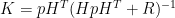
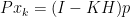
UPDATE EQUATIONS

These equations can look scary as there are many variables so we will now clarify what each variable is.
x,X = These variables represent your state (ie. the things you care about and/or trying to filter). For example, if you are controlling a robotic arm with three joints your state can be:
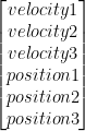
This should be initialized at whatever state you want to start at. If you are treating your start location as the origin than it can be initialized to:
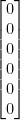
While we like to model and know all states in a system, you should only include states that you need to know. Adding more states can slow the filter and increase uncertainty in the overall state.
u = what ever the action is for the three joint robotic arm the actions can be:

P,p = These numbers represent how confident the filter is with the solution. The best way to do this is to initialize it as a diagonal matrix when the filter runs it will become populated. After running the filter you can look at how the values converge and use them to initialize the filter the next time. The reason it should be initialized as a diagonal is that each entry directly corresponds to the variance of the state in that row so for the above robotic arm with six states the covariance matrix can be initialized as:
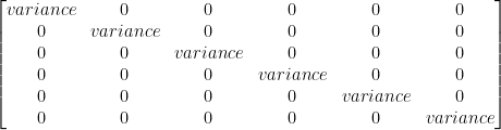
where variance is the square of the standard deviation of the error.
Q= Is the covariance of the process (i.e. action) noise. It is formed similar to the above except that it is a matrix that you determine and does not get updated by the filter. This matrix tells the Kalman filter how much error is in each action from the time you issue the commanded voltage until it actually happens.
K= This matrix gets updates as part of the measurement update stage.
H= Is a model of the sensors, but is hard to determine. An easy approach is to initialize it as a diagonal identity matrix and tweak it to improve the final filter results.
R = Similar to Q except this defines the confidence in each of the sensors. This is the key matrix for conducting sensor fusion
z= These are the measurements that are returned from the sensors at each location. The Kalman filter is usually used to clean the noise from these signals or to estimate these parameters when there is no sensor.
I= an Identity matrix (also diagonal)
The next variables we need to determine are A and B. These matrices are the model that represents how your system changes from one state to the next.
Since the Kalman filter is for linear systems we can assume that if you start at the beginning (t=0) and run your system to the next state(t=1), and run it again(t=2), the amount of change will be the same so we can use that change no matter where (t=wherever) in the system we actually are.
The easiest way to find the A and B matrices is if you are able to collect data from your system by doing experiments before creating the filter with an unforced system (the inputs must be 0). The newState and lastState are both matrices whose columns are the input and output states measured during the experiments. In order for this to work you need to be able to measure the full state, which is often not possible if you are using the Kalman filter as a state estimator (which is a common usage). This allows you to solve for A and B numerically. You need to repeat the experiment n times where n is the dimension of the A matrix.
Since:

then we can rewrite it as:

Following this logic, once you have A you can find B

Knowing the current state, what the last state was, A, and the action that caused the state change you can solve for B.
![B=[x-(A*lastState)]*psudoinverse(action)](https://s0.wp.com/latex.php?latex=B%3D%5Bx-%28A%2AlastState%29%5D%2Apsudoinverse%28action%29&bg=ffffff&fg=000&s=0&c=20201002)
Note: On systems where you are just filtering or fusing inputs (i.e. sensors) than you might not be capable of having any actions so the B*action term cancels and all you need to know is your A term.
When you do not have any prior data then we need a more formal way to determine the A and B matrices. This approach can be difficult and involve a lot of math. The general idea is to start somewhere and perturb your system and record the states, perturb again, record again, etc.
The B matrix can be made in the same way except that instead of perturbing the state we perturb the actions and record the states.
So in pseudocode this would be:
X0 = State you are linearizing about;
U0 = Voltages required to produce (inverse dynamics);delta = small number;
//Finding the A matrix
for ii=1 thru #ofStates{
X=X0;
X(ii)=X(ii)+delta; //perturb state x(i) by delta
X1 = f(X,U0); //f() is the model of system
A(:,ii) = (X1-X0)/delta;
}//Finding the B matrix
for ii=1 thru #ofInputs {
U=U0;
U(ii)=U(ii)+delta; //perturb action U(i) by delta
X1 = f(X0,U); //f() is the model of system
B(:,ii) = (X1-X0)/delta;
}
The f(X0,U) is your model. This model can take a state and an action and determine what the next state will be. This step involves the kinematics and dynamics of the rover. Remember that if your model is not predicting what happens in real life then your model is wrong and you need to fix it!
Now that we know what all of the variables are I want to repeat the algorithm with words. We start with our current state xk-1, your current covariance matrix Pk-1 , and your current input uk-1 to get your predicted state X and predicted covariance matrix p. Then you can get your measurement yk and use the update equations to correct your predictions in order to get you new state matrix xk and the new covariance Pk. Once you do all of that you just keep iterating those steps where you make a prediction and then update the prediction based on some known information.
Advanced Filter Methods
For non-linear system there are two main approaches. The first is to develop an Extended Kalman Filter (EKF). For the EKF you need to linearize your model and then form your A and B matrices. This approach involves a bit of math and something called a Jacobean, which lets you scale different values differently. The second and easier approach is to use piece-wise approximation. For this you break down the data into regions that are close to linear and form different A and B matrices for each region. This allows you can check the data and use the appropriate A and B matrices in the filter to accurately predict what the state transition will be.
Sample Code
Here is the c++ code for a Kalman filter designed for a PUMA 3DOF robotic arm. This code is being used for velocity estimation as this is much more accurate than just differentiating position.
I made bad assumptions for my noise and sensor models to simplify the implementation. I also initialize my covariance as an identity matrix. In my real code I let it converge and save it to a text file that I can read every time I start the filter.
I did this code a long time ago. I am now a bit embarrassed by how the code looks, but I will still share it.
/*******************************************************
* Kalman filter PUMA 3DOF Robotic Arm
********************************************/
#include <fstream>
#include <iostream>
#include <unistd.h>
#include <stdlib.h>
#include <string.h>
#include <stdio.h>
//my matrix library, you can use your own favorite matrix library
#include “matrixClass.h”
#define TIMESTEP 0.05using namespace std;
float timeIndex,m_a1,m_a2,m_a3,c_a1,c_a2,c_a3,tau1,tau2,tau3;
float a1,a2,a3,a1d,a2d,a3d,a1dd,a2dd,a3dd;
float new_a1d, new_a2d, new_a3d;
float TIME=0;
matrix A(6,6);
matrix B(6,3);
matrix C=matrix::eye(6); //initialize them as 6×6 identity matrices
matrix Q=matrix::eye(6);
matrix R=matrix::eye(6);
matrix y(6,1);
matrix K(6,6);
matrix x(6,1);
matrix state(6,1);
matrix action(3,1);
matrix lastState(6,1);
matrix P=matrix::eye(6);
matrix p=matrix::eye(6);
matrix measurement(6,1);void initKalman(){
float a[6][6]={
{1.004, 0.0001, 0.001, 0.0014, 0.0000, -0.0003 },
{0.000, 1.000, -0.00, 0.0000, 0.0019, 0 },
{0.0004, 0.0002, 1.002, 0.0003, 0.0001, 0.0015 },
{0.2028, 0.0481, 0.0433, 0.7114, -0.0166, -0.1458 },
{0.0080, 0.0021, -0.0020, -0.0224, 0.9289, 0.005 },
{0.1895, 0.1009, 0.1101, -0.1602, 0.0621, 0.7404 }
};float b[6][3] = {
{0.0000, 0.0000 , 0.0000 },
{0.0000, 0.0000, -0.0000 },
{0.0000, -0.0000, 0.0000 },
{0.007, -0.0000, 0.0005 },
{0.0001, 0.0000, -0.0000 },
{0.0003, -0.0000, 0.0008 }
};/*loads the A and B matrices from above*/
for (int i = 0; i < 6; i++){
for (int j = 0; j < 6; j++){
A[i][j]=a[i][j];
}
}
for (int i = 0; i < 6; i++){
for (int j = 0; j < 3; j++){
B[i][j]=b[i][j];
}
}/*initializes the state*/
state[0][0]=0.1;
state[1][0]=0.1;
state[2][0]=0.1;
state[3][0]=0.1;
state[4][0]=0.1;
state[5][0]=0.1;lastState=state;
}
void kalman(){
lastState=state;
state[0][0]=c_a1;
state[1][0]=c_a2;
state[2][0]=c_a3;
state[3][0]=a1d;
state[4][0]=a2d;
state[5][0]=a3d;measurement[0][0]=m_a1;
measurement[1][0]=m_a2;
measurement[2][0]=m_a3;
measurement[3][0]=a1d;
measurement[4][0]=a2d;
measurement[5][0]=a3d;action[0][0]=tau1;
action[1][0]=tau2;
action[2][0]=tau3;matrix temp1(6,6);
matrix temp2(6,6);
matrix temp3(6,6);
matrix temp4(6,1);
/************ Prediction Equations*****************/
x = A*lastState + B*action;
p = A*P*A’ + Q;
/************ Update Equations **********/
K = p*C*pinv(C*p*C’+R);y=C*state;
state = x + K*(y-C*lastState);
P = (eye(6) – K*C)*p;
a1=state[0][0];
a2=state[1][0];
a3=state[2][0];
a1d=state[3][0];
a2d=state[4][0];
a3d=state[5][0];
}/* This function is not used since I am using position to get velocity (i.e. differentiation).
* However I think that it is useful to include if you want velocity and position
* from acceleration you would use it */
void integrate(){
new_a1d = a1d + a1dd*TIMESTEP;
a1 += (new_a1d + a1d)*TIMESTEP/2;
a1d = new_a1d;
new_a2d = a2d + a2dd*TIMESTEP;
a2 += (new_a2d + a2d)*TIMESTEP/2;
a2d = new_a2d;
new_a3d = a3d + a3dd*TIMESTEP;
a3 += (new_a3d + a3d)*TIMESTEP/2;
a3d = new_a3d;
TIME+=TIMESTEP;
}/*This gives me velocity from position*/
void differentiation(){
a1d=(state[0][0]-lastState[0][0])/TIMESTEP;
a2d=(state[1][0]-lastState[1][0])/TIMESTEP;
a3d=(state[2][0]-lastState[2][0])/TIMESTEP;
TIME+=TIMESTEP;
}int main () {
initKalman();
char buffer[500];
ifstream readFile (“DATA.txt”); // this is where I read my data since I am proccessing it all offlinewhile (!readFile.eof()){
readFile.getline (buffer,500);
sscanf(buffer, “%f %f %f %f %f %f %f %f %f %f “,&timeIndex,&m_a1,&m_a2,&m_a3,&c_a1,&c_a2,&c_a3,&tau1,&tau2,&tau3);kalman();
differentiation();
//integrate();/*this is where I log the results to and/or print it to the screen */
FILE *file=fopen(“filterOutput.txt”, “a”);
fprintf(file,”%f %f %f %f %f %f %f %f %f %f \n”,TIME,a1,a2,a3,a1d,a2d,a3d,tau1,tau2,tau3);
fprintf(stderr,”%f %f %f %f %f %f %f %f %f %f \n”,TIME,a1,a2,a3,a1d,a2d,a3d,tau1,tau2,tau3);
fclose(file);
}
return 1;
}
Conclusion
This post has focused on implementing a Kalman filter. Hopefully you will be able to take this information to improve and refine your robotic projects. For more information I recommend Greg Welch and Gary Bishops Introduction to Kalman Filtering http://www.cs.unc.edu/~welch/kalman/ and a post from TKJ Electronics.
The Making Embedded Systems podcast has a great discussion on inertial sensors and Kalman filtering that you can listen to.
References
[1] – Maybeck, Peter S. 1979. Stochastic Models, Estimation, and Control, Volume 1, Academic Press, Inc.
[2] – Welsh, Greg. Bishop, Gary. The Kalman Filter. http://www.cs.unc.edu/~welch/kalman/


How tough is it to implement a Kalman Filter on my 5 DOF robotic arm within 12 hours without any prior experience? Also, either way, how should I proceed in learning and implementing it?
Understanding and implementing are two different things, also understanding can of different levels. You can definitely understand enough to just implement KF. Refer :http://robotsforroboticists.com/kalman-filtering/
Hi, thanks. I am a beginner for programming. I want to use sensor fusion like gps and imu using kalman filter. Can you advice how to make it and which programming i can follow?
I always knew that Kalman filters could be explained in more understandable terms. Thanks
Why are you setting a1d in the differentiation function three times?
You are correct it should be a1d, a2d, a3d. I am correcting the code above. Thanks for finding that!
Hello! First thank you for the good explanation about the filter.
Why don’t you take the velocity directly from your state matrix instead of do a differentiation, it is already predicted, didnt it? I have just started to study about this filter and some things are not clear yet. Thank you!
There are 2 steps, the first is where you have an estimate of state in the matrix. However in the second step you want to use your sensor data to update the state estimate. For that you need to differentiate the current sensor data.
Hey there! Thanks for the tutorial. Did you use operator overloading for the matrix multiplication in your matrixClass? Is the class available somewhere?
The variable names: m_a1,m_a2,m_a3,c_a1,c_a2,c_a3,tau1,tau2,tau3,a1,a2,a3,a1d,a2d,a3d,a1dd,a2dd,a3dd
are very cryptic for me. Could you please make them more concrete?
How do the input values look like? Just some floats? I still don´t get how this really works :/
I mean, yes I understand the concepts, but how can I validate if the filter I implement really is improving?
Hi
Great question.
It has been a long time since I wrote this code (and I am a bit embarrassed by it) but I think m_ is an item that was measured by a sensor whereas c_ was something that was computed and gets put into the current state.
The 1, 2 or 3 represent the different joints in this arm (it was a 3 jointed robotic arm).
The d’s at the end were differentiations of the position. So:
a1 = position
a1d = velocity
a1dd = acceleration
tau is the action (my control) of each of the 3 joints.
The matrix class used operator overloading. Unfortunately it is not public so I can not share that matrix class.
The inputs are just floats either based on measured values or the commands that I send each joint.
Validation will depend on the situation. In the easy case where you are estimating a parameter (say position) that you can measure afterwards you can plot your estimate and actual position. The closer your estimate is to the actual the better. You can do this multiple times while changing your filter until the two lines converge on top of each other.
Thank you very much!
Thanks. Can you give a bit more detail on how the transition Matrix A is created. You reference doing this experimentally, but I got lost a bit on this.
In almost every academic tutorial, A is some simplified version of the identity matrix with a few of the off diagonal elements filled in for velocity so I’m very interested in any details you can provide regarding this more ‘practical’ state transition matrix.
Hi
You are correct with how to start the A matrix. If you have prior data you can precompute for a better A to start your filter with.
To do that you run a loop with pre-collected data. where you can keep updating A based on:
A=newState * psudoInverse(priorState)
I generally use the psuedo inverse in case the priorState matrix is singular.
Checkout https:// github.com/dr-duplo/eekf. I made a small efficient library for an Extended Kalman Filter.
Nice! Great resource.
Hey..I’ve been trying to estimate altitude from barometer(measured) and accelerometer(predicts)..so how do I find the covariance matrix considering I know the error in accelerometer..how do I find error in position and velocity.?
Hi, thanks for the explanations !
I want to use the code but I don’t get how you get the C and R matrix modified and/or initialised ?
Thank you very much for sharing it, it’s a great tuorial.
Could you please upload the “Data.txt” file?….that would be great help.
Thanks. Unfortunately I no longer have data.txt. I used this code about 8 years ago.
Hi, thanks for this effectual tutorial, it clarified me a lot. I have to implement Kalman Filter for estimating position based on acceleration, so i have two uncertainties. First of these is that I don’t understand what we can use for input in prediction stage for control input? Are these values have to modeling real world motion, for example if I estimate position, these values have to be something similar to real world acceleration or what? And the second one is what can I pass through the Kalman filter? Do i have to find displacements double integrating accelerations and then to use that values in Kalman filter? or maybe first to obtain filtered accelerations values and then double integrating it? Thanks in advance, and again thank you for this great post.
Your inputs would generally be something that can be used to compute the desired output. For example for position you could use velocity, accelerations, etc..
You can go in either direction.
Double integration of sensor data is very prone to serious errors. Even a very small DC offset can cause the data to be unusable.
Thanks for the post. It is really helpful however I also have the same questions as Milan. Anyone knows, can help us to understand more. Thank you!
See above
Pingback: Software that Forms a Robot - Robots For Roboticists
Thanks for the article David. For those looking for a more in depth treatment of the individual Kalman filter matrices, check out the article I wrote:
https://buddingroboticist.wordpress.com/2017/06/14/an-implementers-guide-to-the-kalman-filter/
I go through a thorough example of how to design every matrix in a KF.
Updated link:
https://makingthingsmove.wordpress.com/2017/06/14/an-implementers-guide-to-the-kalman-filter/
Q= Is the covariance of the process (i.e. action) noise. It is formed similar to the above except that it is a matrix that you determine and does not get updated by the filter. This matrix tells the Kalman filter how much error is in each action from the time you issue the commanded voltage until it actually happens.
I am just curious why the matrix is not necessarily updated?
Is there any chance you still have your matrixClass.h or point me to an equivalent version?
Hi
Sorry It has been to long and I no longer have it. If you search google there are plenty of options.
Hi,
it seems that
measurement[0][0]=m_a1;
measurement[1][0]=m_a2;
measurement[2][0]=m_a3;
measurement[3][0]=a1d;
measurement[4][0]=a2d;
measurement[5][0]=a3d;
are not used.
Shouldn’t they be used as y ?
(instead of y=C*state;)
Regards
Dear David,
Thanks for your explanation on KF and the example code!!!